
The case for WAR
How a common baseball metric can help us find value in fantasy football

Wow! First off I want to say welcome to all of the new readers, most of whom have come recommended by . If any of you who read this newsletter haven’t tried out college fantasy football and/or aren’t subscribed to the VolumePigs Substack, I encourage you to change that! He is one of the hardest working analysts in the space and consistently finds your inbox with excellent content on the next studs at the NCAA level.
For those of you who are new here, here’s a little background so you know what to expect. I started the Working Through Regressions Substack back in January as a way to put the thoughts in my head on paper and share them with friends who are also interested in fantasy football. I make my living as an engineer, but most of my hobbies have something to do with sports, so this is the perfect bridge. I’ve dug into a few different topics so far during the offseason, and I’ll continue to evolve as we shift in season. I focus exclusively on the NFL, that said, I like to study things from a theory/statistical approach (you’ll get a good taste of that in this post) so I’m hopeful the concepts can be applied to multiple formats.
Intro
The MLB is lightyears ahead of the NFL when it comes to analytics, and rightfully so, it is a very binary game. 90% of the result is determined by a single matchup between two players. Therefore, it’s much simpler to determine the outcome of a given play compared to the dynamic nature of an NFL game where you have 11 players on each side of the ball, all involved in the play in some manner often before the ball is even snapped. One common metric from baseball that has made it’s way to fantasy football in recent years is Wins Above Replacement (WAR). In short, WAR attempts to calculate how many games a team will win by starting a particular player vs the average replacement player.
To extend this to fantasy football, you could calculate the average number of points scored in your league for each week, then calculate the average number of points a replacement player scores each week for each starting roster spot. Depending on whose definition you are reading, you can also apply some distribution to the expected points to account for week-to-week variability. The difference gives you the expected number of wins for a replacement lineup. Then take a particular player, say Justin Jefferson, and plug him in place of the replacement WR, and calculate the number of expected wins this time with Justin Jefferson. The difference in expected wins with Jefferson vs the expected wins with the replacement player is his WAR.
Is your head spinning yet? Yeah, mine too.
As you can tell the computation gets complex pretty quickly. More importantly, it depends entirely on your specific league settings which makes it difficult to apply to everyone reading this. I want to keep things a little simpler so I’ll modify WAR slightly to what’s often referred to as value over replacement player (VORP).
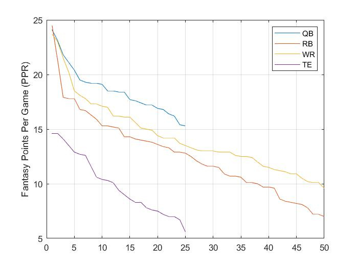
The above graph shows points per game for the top 25 QBs and TEs, and the top 50 RBs and WRs. Ironically, this past year Josh Allen, Christian McCaffrey and Tyreek Hill were all within 1 point from each other in terms of PPG, so that makes this a fun exercise. Among the three, who was the most valuable? Who would’ve given you the best chance of winning your league?
Or you could ask more generally, based on this information, what position is most valuable? How do you compare QB to RB, or RB to TE, and so on, when the scoring at each position is so different? At first glance, it doesn’t seem crazy to think QB is the most valuable because they score the most points, then WR, RB, and finally TE. That’s where VORP can be a useful tool to help answer these questions.
What is VORP?
First, we have to define what a “replacement” player is. Let’s start with a pretty standard 12-team PPR league with 1QB, 2RB, 2WR, 1TE and 1 Flex. I’ll skip K and DST. Let’s assume each team has a player within the top-12 for QB and TE. For RB and WR, one top-12 and one in the 13-24 range. Finally, for the flex, we’ll take the next 12 highest scoring players after the top-24 RBs/WRs and top-12 TEs are removed.
If you consider these guys the starters, the remaining players are either on your bench or available on waivers. Those remaining players are the replacement player. They are the player you would start in the situation you can’t play your usual starter because of injury or bye week.
For this example league, here’s how the average starter and replacement scoring worked out in 2023:
QB — Starter: 20.32 PPG, Replacement: 17.13 PPG, Delta: 3.19
RB — Starter: 15.68 PPG, Replacement: 11.18 PPG, Delta: 4.50
WR — Starter: 17.10 PPG, Replacement: 11.53 PPG, Delta: 5.57
TE — Starter: 12.33 PPG, Replacement: 8.07 PPG, Delta: 4.26
The delta is the number we should be paying the most attention to, that is the average VORP for the position. You can start to see pretty quickly the difference between the average starter and replacement for QB is small compared to the other positions, especially WR.
Why is this important?
Going back to the example league, if there are 12 teams and you can only start one QB, there are probably somewhere around 18 QBs that are rostered. Some teams will carry two, others will only carry one. So, a guy like Kirk Cousins (19.3 PPG) would be rostered, while Sam Howell (16.8 PPG) might not be. If you’re not getting an elite QB, why use a high-vale pick when you can get a replacement QB that’s only a couple points worse for pennies? This is the foundation of the late-round QB strategy.
This idea can be visualized in the graph too. In the example I just gave, Kirk Cousins was QB7 in PPG, and Sam Howell was QB21. The takeaway is this — the bigger the drop-off from one player to the next, the more valuable the player before the drop-off is. Or, the steeper the slope, the more important the position. After about QB6, once the elite mobile QBs are gone, you’re better off waiting.
But… if RB has the steepest slope, why does WR have the biggest delta between starter and replacement? That’s because of the Flex position. Remember back to the definition of a replacement player, the Flex was defined as the next 12 players after the RBs, WRs and TEs were removed. Because WRs score more points on average, 11 of the 12 flex spots were WRs. So the replacement RB started at RB26 while the replacement WR started at WR36. You could still argue having the RB1 is more valuable than the WR1, and I wouldn’t disagree, but that doesn’t apply for the position as a whole.
How to apply VORP?
If we put things in the perspective of VORP, you can see now that in terms of importance the positions are a bit flipped compared to scoring. Despite being the highest scoring position in fantasy, QB is the least valuable in single-QB leagues.
If you wanted to use VORP in your fantasy draft, you could easily just take the 12 players with the highest VORP and consider that round 1 guys, then the next 12 for round 2, and so on. With that idea in mind, here’s what I found:
Round 1 — 6 WRs, 5 RBs, 1 QB
Round 2 — 5 WRs, 4 TEs, 2 RBs, 1 QB
Round 3 — 5 WRs, 3 RBs, 3 TEs, 1 QB
Round 4 — 5 RBs, 4 WRs, 2 QBs, 1 TE
Round 5 — 5 RBs, 4 WRs, 2 TEs, 1 QB
As you can see, WRs dominate the early rounds. Surprisingly, there were four TEs in round 2, then another three in round 3. Once you start getting into the middle rounds, RBs start becoming more valuable. And finally, there are a few QBs scattered across each of the first five rounds.
Is the market pricing TEs appropriately?
If you believe in VORP, even as just a baseline method for valuing players/positions, it would tell you TEs are being massively mispriced right now. We just saw from the 2023 results, if everyone drafted optimally, there would’ve been seven TEs taken before the 3rd round closed. Looking at current Underdog ADP, the TE1, Sam LaPorta, has an ADP of 35.8! So there should be seven TEs before pick 36 and we’re barely getting 1?!
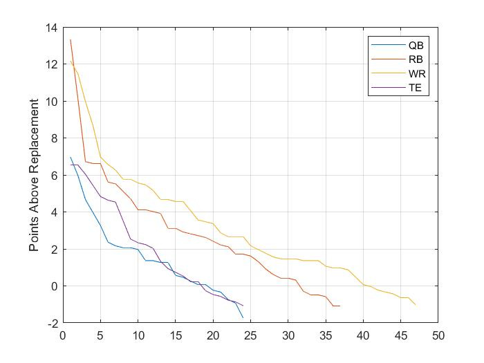
Referring back to the points above replacement chart, the other three positions drop off quickly from the top 1 or 2 players, whereas TE doesn’t see a cliff until TE7. The takeaway is don’t be left without one of those top-7 guys, which should be easy considering how late they’re being drafted.
What about the RB dead zone?
If there are 10 RBs between round-4 and round-5 wouldn’t this counter the idea of the dead zone? The caveat to all of this is that VORP doesn’t consider draft position.
The 5 RBs with round-1 VORP were: Christian McCaffrey, Kyren Williams, Alvin Kamara, Raheem Mostert, and De’Von Achane. CMC was the only player who actually had round-1 ADP, Alvin Kamara was in the dead zone, and the rest were drafted after the dead zone. So this actually supports the argument to avoid the dead zone, or at least the dead zone profile I discussed in the last post.
Here were the 6 WRs with round-1 VORP: Tyreek Hill, CeeDee Lamb, Keenan Allen, Amon-Ra St. Brown, Justin Jefferson, and AJ Brown. Everyone knew these guys were the superstars before the season started. Keenan Allen was the only one without round-1 ADP.
So, if you read my WR stats review post, this shouldn’t be a surprise to you. WRs are the most predictable position, and you should absolutely prioritize them in the early rounds of your draft.
Conclusion
I don’t expect this to be the law on how to draft, but I do believe the importance of knowing how players are being valued versus how they should be valued before jumping into the draft room cannot be overstated. This approach gives us a good starting point for that.
With redraft leagues just around the corner, August will be dedicated to covering some popular draft strategies using a lot of the principles discussed here.